Lattice Points in High-Dimensional Spheres

(Lattice points in spheres.)

— THE GENERALIZED GAUSS PROBLEM —

Gauss proved in 1834 that the number of lattice points contained in a circle of radius $R$ is well-approximated by the area of the circle, $\pi R^2$ . But just how good is this approximation, exactly? To be concrete, let $S_2(n)$ denote the number of lattice points contained in the circle of radius $\sqrt{n}$ . Gauss proved that

$\displaystyle S_2(n) = \pi n + O \left(n^\frac{1}{2}\right),$

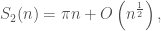
and the Gauss Circle Problem is the conjecture that this exponent $\frac{1}{2}$ might be improved to $\frac{1}{4}+\epsilon$ for any $\epsilon > 0$ .

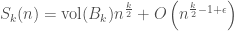
In higher dimensions, we similarly expect (and can prove!) that the number of lattice points $S_k(n)$ in the $k$ -dimensional sphere of radius $\sqrt{n}$ is asymptotic to the volume of that sphere. As for the error in that approximation, the analogous generalized Gauss Circle Problem is the conjecture that

$\displaystyle S_k(n) = \mathrm{vol}(B_k) n^\frac{k}{2} + O\left(n^{\frac{k}{2}-1+\epsilon}\right)$

for all $k \geq 3$ , where $B_k$ is the $k$ -dimensional ball of radius 1. (Note that our conjecture differs from the 2-dimensional case.)

We often find that geometric problems simplify in higher dimensions. This case is no exception, as the generalized Gauss Circle Problem has already been solved in dimensions four and greater.

A key idea in these proofs is geometric — lattice points become spread quite uniformly over the sphere in higher dimensions. (See here, pg. 8 for more comments.) However, it’s possible to prove some of these results using purely analytic means, and it’s a good exercise to do so, as understanding the Gauss Circle Problem from many angles may lead to a solution in the last outstanding cases.

In this note, I give a short analytic proof of the generalized Gauss Circle Problem in dimension six via L-functions. This proof readily generalizes to larger even dimensions and casts some low-dimensional obstructions in an interesting light.

— A PROOF IN SIX DIMENSIONS —

The lattice-point-counting function $S_6(n)$ may be written as a partial sum,

$\displaystyle S_6(n) = \sum_{m \leq n} r_6(n),$

in which $r_6(m)$ is the number of lattice points on the sphere of radius $\sqrt{n}$ . From the equation of the sphere, $x_1^2+ \ldots x_6^2 = n$ , we see that $r_6(m)$ is exactly the number of ways to represent $n$ as a sum of six squares.

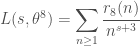
Consider the generating function $\sum r_6(n) q^n$ , where $q= e^{2\pi i z}$ . As a function this is exactly $\theta^6(z)$ , the sixth power of one of the classical Jacobi theta functions. As such, it is a modular form of weight 3 (and level 4, with character) and may be written as a linear combination of (twisted) Eisenstein series. Equating coefficients gives the identity

$\displaystyle r_6(n) = 16 \sum_{d \mid n} \chi(d) \left(\frac{n}{d}\right)^2-4\sum_{d \mid n} \chi(d) d^2= 16(\chi \star N^{2})(n) - 4 n^2(\chi \star N^{-2})(n),$

in which $\chi$ is the non-trivial character mod 4 and $\star$ represents Dirichlet convolution. (Related identities of this form can be found here.)

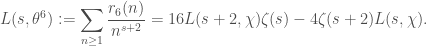
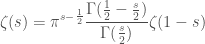
From here we obtain a strange proof of the fact that every positive integer may be written as a sum of six squares (if we squint hard enough), as well as a convenient closed-form for the L-function $L(s,\theta^6)$ :

$\displaystyle L(s,\theta^6):=\sum_{n \geq 1} \frac{r_6(n)}{n^{s+2}} = 16 L(s+2,\chi)\zeta(s) -4\zeta(s+2)L(s,\chi).$

We now apply Perron’s Formula to derive an analytic expression for the partial sum of the coefficients $r_6(n)$ . Since Perron’s Formula takes many forms and most are technical, I’ll include one here for reference. [This particular version is stolen from one of Terry Tao’s blogposts.]

Theorem (Truncated Perron, Prop. 12): Suppose that the Dirichlet series given by $\sum a(n) n^{-s}$ satisfies $a(n) = O(\log(n+2))$ for all $n$ . Choose $X \geq T \geq 2$ . For $\sigma = 1+1/\log X$ we have

$\displaystyle \sum_{n \leq X} a(n) = \frac{1}{2\pi i} \int_{\sigma -iT}^{\sigma+i T} \sum_{n =1}^\infty \frac{a(n)}{n^s} X^s \frac{ds}{s} + O\left(\frac{X}{T} \log^2(XT)\right).$

From the estimate $\sigma(n) \ll n\log\log(n)$ known as Grönwall’s Theorem (not to be confused with Grönwall’s Inequality) and the convenient formula

$\displaystyle r_4(n) = 8 \sigma(n) - 32 \sigma\left(\frac{n}{4}\right)$

(see here), we conclude that $r_4(n) \ll n \log\log n$ . Then, since

$\displaystyle r_5(n) = \sum_{m^2 \leq n} r_4(n-m^2) \ll \sqrt{n} r_4(n)$ ,

we see that $r_5(n) \ll n^{3/2} \log \log n$ . A second application of this recursion implies that $r_6(n)/n^2 \ll \log(n)$ , hence our Theorem applies. It follows that

$\displaystyle \sum_{n \leq X} \frac{r_6(n)}{n^2} = \frac{2}{\pi i} \int_{\sigma-iT}^{\sigma+iT}\!\!\big(4L(s+2,\chi)\zeta(s)-\zeta(s+2)L(s,\chi)\big) X^s \frac{ds}{s} +O\left(\frac{X}{T} \log^2(XT)\right).$

To treat the integral, we shift the contour of integration to $\sigma =-\frac{1}{2}$ and extract residues. We encounter a residue at $s=1$ from $\zeta(s)$ which looks like

$16L(3,\chi)X$

as well as a pole at $s=0$ which contributes $O(1)$ . (There is some contribution from the `horizontal’ parts of our contour shift which is likewise small.)

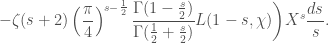
With the functional equations for the Riemann zeta function (eq. 14) and the Dirichlet L-function $L(s,\chi)$ ,

$\displaystyle \zeta(s) = \pi^{s-\frac{1}{2}} \frac{\Gamma(\frac{1}{2}-\frac{s}{2})}{\Gamma(\frac{s}{2})}\zeta(1-s)$

$\displaystyle L(s,\chi)= \left(\frac{\pi}{4}\right)^{s-\frac{1}{2}} \frac{\Gamma(1-\frac{s}{2})}{\Gamma(\frac{1}{2}+\frac{s}{2})} L(1-s,\chi),$

we transform our shifted integral into

$\displaystyle \frac{4}{2\pi i} \int_{-\frac{1}{2}-iT}^{-\frac{1}{2}+iT}\!\bigg(4\pi^{s-\frac{1}{2}} \frac{\Gamma(\frac{1}{2}-\frac{s}{2})}{\Gamma(\frac{s}{2})}\zeta(1-s)L(s+2,\chi)$

$\displaystyle \hspace{3 mm}-\zeta(s+2)\left(\frac{\pi}{4}\right)^{s-\frac{1}{2}} \frac{\Gamma(1-\frac{s}{2})}{\Gamma(\frac{1}{2}+\frac{s}{2})} L(1-s,\chi)\bigg) X^s \frac{ds}{s}.$

A naïve bound in absolute value using Stirling’s approximation and boundedness of L-functions in their convergent half-planes shows that this integral is no larger than

$\displaystyle \int_{-T}^T \vert t \vert^{0} \cdot X^{-\frac{1}{2}} dt \ll X^{-\frac{1}{2}} T.$

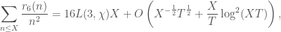
By the method of stationary phase we recognize that spin in the integrand leads to a certain amount of cancellation in $T$ -growth, reducing our $T$ -dependence down to $\sqrt{T}$ . (Here, this spin comes from the gamma ratios.) We conclude that

$\displaystyle \sum_{n \leq X} \frac{r_6(n)}{n^2} = 16L(3,\chi) X + O\left( X^{-\frac{1}{2}} T^{\frac{1}{2}}+ \frac{X}{T} \log^2(X T)\right),$

and by taking $T = X$ these errors contribute $O(\log^2 X)$ overall.

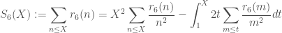
Of course, now that we understand the Perron integral, we can recover $S_6(n)$ by Abel’s summation formula (ie. summation by parts). Specifically,

$\displaystyle S_6(X):=\sum_{n \leq X} r_6(n) = X^2 \sum_{n \leq X} \frac{r_6(n)}{n^2} - \int_1^X 2t\sum_{m \leq t} \frac{r_6(m)}{m^2} dt$

$\displaystyle \,\hspace{2 mm}= 16L(3,\chi) X^3 - \int_1^X 32L(3,\chi) t^2 \,dt+ O\left(X^{2}\log^2 X\right).$

We conclude that

$\displaystyle S_6(X) = \tfrac{16}{3} L(3,\chi) X^3 + O\left(X^{2}\log^2 X\right),$

which proves the generalized Gauss Circle Problem in dimension six, as our error bound matches the optimal error bound given above.

Remark — Since our main terms must agree with known results, we see that

$\displaystyle \tfrac{16}{3} L(3,\chi) = \mathrm{vol}(B_6) =\tfrac{\pi^3}{6}$

for free. To verify this equality independently, we compute

$\displaystyle L(3,\chi) = \sum_{n=0}^\infty \frac{1}{(4n+1)^3} - \sum_{n=0}^\infty \frac{1}{(4n+3)^3} = \frac{\pi^3}{64}+\frac{7\zeta(3)}{16}-\left(\frac{7\zeta(3)}{16}-\frac{\pi^3}{64}\right)=\frac{\pi^3}{32}$

with the help of a CAS or the online tool wolfram|alpha, then simplify.

— PROVING THE GAUSS CIRCLE PROBLEM IN OTHER DIMENSIONS —

The method outlined above in dimension $k=6$ readily generalizes to any larger even dimension, since $L(s,\theta^{k})$ always admits a closed form in terms of $L(s,\chi)$ , $\zeta(s)$ , and an L-function attached to a cusp form when $k$ is even. (See here for more formulas related to sums of an even number of squares.)

When the dimension is odd this handy factorization does not exist and this technique fails to apply. (This is because odd powers of the theta function lack Euler products.)

In dimensions two and four our method fails despite the existence of the closed forms

$\displaystyle \sum_{n \leq X} r_2(n) = \frac{2}{\pi i} \int_{\sigma-iT}^{\sigma+i T} \zeta(s) L(s,\chi) X^s \frac{ds}{s} + O\left(\frac{X}{T} \log^2(XT)\right)$

$\displaystyle \sum_{n \leq X} \frac{r_4(n)}{n} = \frac{4}{\pi i} \int_{\sigma-iT}^{\sigma+iT}\zeta(s)\zeta(s+1)\left(1-4^{-s}\right) X^s \frac{ds}{s}+O\left(\frac{X}{T} \log^2(XT)\right).$

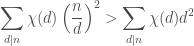
Here, we observe that in the case $k=2$ the product $\zeta(s)L(s,\chi)$ has no separation of arguments, and for $k=4$ our arguments are separated by $1$ . (In the case $k=6$ we have a shift of $2$ , and so forth.) When the shift strictly exceeds $1$ , as happens for $k>4$ , we can move both series into their convergent half-planes at the same time by reflecting one series or the other with functional equations.

It may be possible to salvage the $k=4$ case with a great deal of technical work, since our separation in that case is exactly $1$ and any improvement would be sufficient. (It hardly seems worth it, though, since other methods can prove this result with very little work. See Exercise 3.) For the case $k=2$ , the original Gauss Circle Problem, this method is certainly useless.

— EXERCISES —

Exercise 1: Prove that

$\displaystyle \sum_{d \mid n} \chi(d) \left(\frac{n}{d}\right)^2 > \sum_{d \mid n} \chi(d) d^2$

and conclude that every positive integer may be written as a sum of six squares. (If we just wanted the result, it would be easier to show that $r_4(n)>0$ and apply that result.)

Exercise 2: Let $d(n)$ denote the number of divisors of $n$ . Prove that

$\displaystyle d(n) = O\left(n^\epsilon\right)$

for all $\epsilon > 0$ . Prove that $d(n) \neq O\left( \log n\right)$ . (This is one respect in which the sum-of-divisors function $\sigma(n)$ is more regular than $d(n)$ .)

Exercise 3: Use the average order result

$\displaystyle \sum_{n \leq X} \sigma(n) = \frac{\zeta(2)}{2} X^2 + O\left( X \log X \right)$

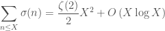
(Thm 3.4 in Apostol’s Introduction to Analytic Number Theory, eg.) and the expression for $\sigma(n)$ following Perron’s Theorem to prove the Gauss Circle Problem in dimension 4.

Exercise 4: Find an alternate expression for the L-function

$\displaystyle L(s,\theta^8) = \sum_{n \geq 1} \frac{r_8(n)}{n^{s+3}}$

and prove the generalized Gauss Circle Problem in dimension 8.

Exercise 5: Since $S_2(n) \sim \pi n$ from Gauss, we see that the average value of $r_2(n)$ is $\pi$ , despite the fact that `most’ integers cannot be represented as a sum of two squares. Use our analytic formula for $S_2(n)$ to write this average value in terms of $L(s,\chi)$ and derive the Gregory series,

$\displaystyle \frac{\pi}{4} = 1-\frac{1}{3} + \frac{1}{5} - \frac{1}{7}+ \frac{1}{9} - \ldots$

a. w. walker

mathematics and miscellany

Lattice Points in High-Dimensional Spheres

Leave a Reply Cancel reply

Share this:

Like this:

Leave a Reply Cancel reply