
 Lagrange’s Four Square Theorem (Lagrange, 1770) is the well-known result that every positive integer can be written as the sum of four integer squares. This was strengthened by Legendre’s 1797-1798 proof of the similar-sounding Three Squares Theorem, which proved that an integer

Since either 
For sums of two squares the chronology is a bit murkier. Fermat (being Fermat) claimed a proof of the classification of these numbers in 1640, but there’s no evidence that Fermat ever had a proof to back up his claims. Thus the following classification is credited to Euler, who worked on the problem between 1747 and 1749.
Theorem (Euler): A positive integer 
Lagrange’s Four Square Theorem obviously implies that any integer can be written as a sum of five squares, or six squares, etc. As for the classification of integers expressible as a sum of one square – consider it an exercise for the reader.
— DENSITY —
In this post I’d like to describe these theorems in a different light, through the language of density. Unfortunately, since the integers have no uniform measure, we’ll have to be a bit careful with what we mean by this.
To state our questions clearly we introduce some notation from additive number theory. If 


Let 


which implies that the densities of these sets (if they exist) should be non-decreasing. Moreover, if 
![\displaystyle\sigma(A):= \lim_{n \to \infty} \frac{\#(A \cap [1,n])}{n},](https://s0.wp.com/latex.php?latex=%5Cdisplaystyle%5Csigma%28A%29%3A%3D+%5Clim_%7Bn+%5Cto+%5Cinfty%7D+%5Cfrac%7B%5C%23%28A+%5Ccap+%5B1%2Cn%5D%29%7D%7Bn%7D%2C&bg=ffffff&fg=444444&s=0&c=20201002)
(when the limit exists), then clearly 

The classification of sums of three squares by Legendre makes calculation of 


are disjoint, and can therefore compute the density of

This bounds the density 
![[0,5/6]](https://s0.wp.com/latex.php?latex=%5B0%2C5%2F6%5D&bg=ffffff&fg=444444&s=0&c=20201002)

serves to bound 
To compute the actual value of

This density can be thought of as a regularized upper density, in the sense that 
While not a viewpoint that we’ll need here, we point out that both 

![[1,N]](https://s0.wp.com/latex.php?latex=%5B1%2CN%5D&bg=ffffff&fg=444444&s=0&c=20201002)


The Dirichlet density is generally preferable to the upper density when the set you are studying has underlying multiplicative structure. In light of Euler’s theorem on the sums of two squares, this is certainly the case for
— COMPUTING THE DENSITY OF
Let 

Here we see how well the Dirichlet density suits this problem, as the Riemann zeta functions cancel out in the definition of 
To motivate our next step, it makes sense to pause and develop heuristics for what we expect the density of 


- Large integers
- Primes are equidistributed among the residues 1 and 3 mod 4.
- Primes in the square-free part of
Together, these heuristics suggest that an `average’ large integer
We therefore claim that 

we need only prove that the harmonic series of primes congruent to 3 mod 4 diverges. Yet this is a special case of the strong form of Dirichlet’s Theorem (below), which proves our claim that 
Theorem (Dirichlet, 1837): Fix positive, coprime integers 


Dirichlet’s Theorem predates the Prime Number Theorem (PNT) by 59 years and is often regarded as the genesis of modern analytic number theory. And, unlike the PNT, Dirichlet’s Theorem avoids many of the technical details that obscure the role of L-functions in its proof.
To keep this post self-contained and finite I will not include a full proof of Dirichlet’s Theorem. Rather, I will illustrate Dirichlet’s Theorem in the simple case 

— DIRICHLET’S THEOREM IN A SIMPLE CASE —
Theorem: The harmonic sum of primes congruent to 1 mod 4 diverges. In particular, there are infinitely many primes congruent to 1 mod 4.
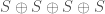
Proof: We introduce the Dedekind zeta function 

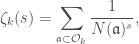
where the sum exhausts the non-zero ideals 

![[\mathcal{O}_k : \mathfrak{a}]](https://s0.wp.com/latex.php?latex=%5B%5Cmathcal%7BO%7D_k+%3A+%5Cmathfrak%7Ba%7D%5D&bg=ffffff&fg=444444&s=0&c=20201002)
![k = \mathbb{Q}[i]](https://s0.wp.com/latex.php?latex=k+%3D+%5Cmathbb%7BQ%7D%5Bi%5D&bg=ffffff&fg=444444&s=0&c=20201002)
![\mathcal{O}_k = \mathbb{Z}[i]](https://s0.wp.com/latex.php?latex=%5Cmathcal%7BO%7D_k+%3D+%5Cmathbb%7BZ%7D%5Bi%5D&bg=ffffff&fg=444444&s=0&c=20201002)

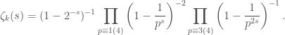
as in Euler’s factorization of the Riemann zeta function. The classification of prime ideals 
![\mathbb{Z}[i]](https://s0.wp.com/latex.php?latex=%5Cmathbb%7BZ%7D%5Bi%5D&bg=ffffff&fg=444444&s=0&c=20201002)

- if
, then
factors into a product of two Gaussian primes of norm
- if
, then
remains prime in
;
- the prime 2 factors as
.
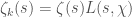
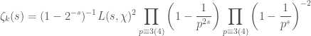
It follows that
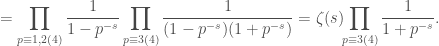
Since 

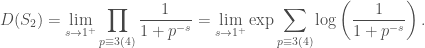
On the other hand, the 2-factor and the second infinite product in (2) converge as

which implies that the harmonic series of primes congruent to 

— EXERCISES —
Exercise 1: What is the average number of ways an integer can be written as the sum of two squares? What about three squares or four squares?
Exercise 2: Let 


Exercise 3: Our proof that 

Exercise 4: Let
holds in the half-plane 

Pingback: Lattice Points in High-Dimensional Spheres | a. w. walker·
I am now not positive where you are getting your information, but good topic. I needs to spend a while finding out more or figuring out more. Thank you for fantastic info I was looking for this info for my mission.
LikeLike