

(Image credit David Zerba, 2013)
— GRAPHS OF LARGE GIRTH —
To refresh on a bit of graph theory, we define a k-regular graph to be a graph in which every vertex has k neighbors. Thus 0-regular graphs are collections of disconnected vertices, while 1-regular graphs consist of disconnected edges. A 2-regular graph consists of disconnected cycles (or perhaps infinite chains, if the graph is infinite).
For a general graph 


The story is quite changed if we consider finite k-regular graphs with 


and Erdős and Sachs showed that logarithmic growth (with a constant worse than 2) is actually attainable. The best known constant in these estimates is currently 4/3, as happens for certain trivalent sextet graphs and for the Ramanujan graphs of Lubotzky, Philips, and Sarnak. (In particular, it’s not known whether or not the constant 2 is sharp.)
A construction due to Brooks and Makover relates graphs of large girth to hyperbolic surfaces of large systole. (Here, the systole of a hyperbolic surface is the shortest homotopically non-trivial (and non-peripheral) loop on the surface.) This construction is perhaps unsurprising, since the dual graph of a surface triangulation is 3-regular.
— BOUNDING THE NUMBER OF MATRICES OF SMALL TRACE —
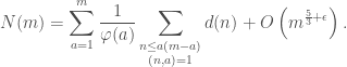
In 2016, Bram Petri and I submitted a paper that builds upon the machinery of Erdős and Sachs to construct a family of genus 
(This lower bound on the size of the systole is sharp up to constants.)
A key ingredient in our paper (and where I, as a number theorist, finally made myself useful) is a count of 


This will actually be infinite for 

for all 


Proposition 1 (PW, Proposition 3.2): For 

Here, the trivial bound 


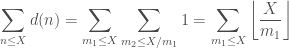
For averages of divisor sums over linear polynomials, far more is known. In the absolute simplest case, we have

for some 


Fortunately for Bram and me, a bound for the partial sums of

The trivial bound 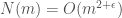


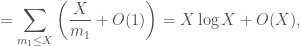
The first term is 

as a consequence of the fact that the divisor function equidistributes over the (primitive) residue classes.
Tracking the propagation of this error term and adjusting some limits of summation for simplicity, we see that
The next step in our evaluation is estimation of the inner sum. If we open up the inner sum in the line above we see that

The innermost sum just counts the number of integers less than 


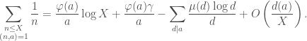
Proposition 2: We have

Proof: (See here, as well.) Standard tricks give

in which 


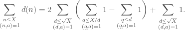
If you’re just looking for a slightly-improved upper bound (as was the case in my paper with Bram), it’s enough to bound the inner sum in (2) via Proposition 2 and write

Ignoring coprimality in the 


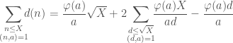
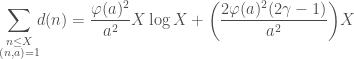
Theorem 3 (PW, Proposition 3.4): We have 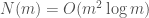
— DIRICHLET’S HYPERBOLA METHOD —
There’s some clear room for improvement here, and while looking over this paper recently I decided to see what could be shown with a little more work. The core inefficiency in the previous section concerns the way we opened up the divisor sum

in line (2). In essence, our treatment resembles the calculation

which gives a quick proof of the fact the main term in (1) is 
As it happens, our problem can be solved using the same tool that Dirichlet used to extract refined asymptotics in (1): the hyperbola method. (So-called because divisors of 
Very briefly, the hyperbola method exploits the 


Here, the inner sum of the double sum counts the number of lattice points 


With some bookkeeping, we realize that a similar statement holds for the sum over 
Applying Proposition 2 gives

To handle the two terms that appear in the sum at right in (3), we require two variants of Proposition 2. This first follows from Proposition 2 and partial summation, and we state it without proof:

The proof of the other fact we’ll need is different enough that we state it as a Lemma. The proof is similar to Proposition 2 and is hinted in the exercises below.
Lemma 4: We have
Proof: See the Exercises.
Simplification of the sums in (3) produces an estimate for the restricted partial sums of divisors in the spirit of Dirichlet’s hyperbola method:

Heuristically, we consider the factors 


— ASYMPTOTICS FOR MATRICES OF BOUNDED TRACE —
Now that we have a good estimate for sums of divisors over the integers coprime to
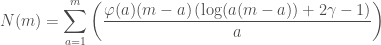

The first term at right in (4) represents the dominant contribution towards
To handle the simplified partial sum of 

(Better error bounds are known but this is more than sufficient.) Thus the first term in (4) grows as


The double sum in (4) may be simplified by reversing the order of summation. Splitting 

To simplify further, we note that

in which we’ve used that 

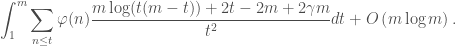
It’s unclear what the optimal error should be in this expression. Certainly our error exceeds 


A plot of the error term for 


— EXERCISES —
Exercise 1: Prove Lemma 4 by modifying Proposition 2 and applying the estimate
Exercise 2: By reversing the order of summation, prove that

Exercise 3: Prove that

and apply the Cauchy-Schwarz inequality to prove that 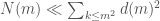
Exercise 4: Prove that

Conclude using Exercise 3 that 

Pingback: Two Classic Problems in Point-Counting | a. w. walker·