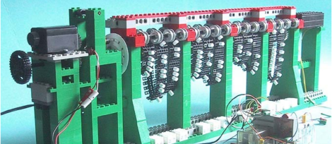
Instructive Examples in Kraitchik’s Method

A Lehmer Sieve made of LEGO. The pins represent quadratic residues.

In his excellent and excellently-named expository piece A Tale of Two Sieves, Carl Pomerance tells the history of two factoring algorithms, the quadratic and number field sieves. This story begins with a factorization technique called factorization via congruence of squares, which attempts to factor $N$ by constructing a non-trivial congruence of the form $a^2 \equiv b^2 \!\! \mod N$ .

If such a congruence is known, then $N \mid (a-b)(a+b)$ , and the factors of $N$ distribute between $(a-b)$ and $(a+b)$ . If we’re lucky (or at least, not unlucky), each of $a-b$ and $a+b$ gets at least one prime factor of $N$ and we can detect such a factor by computing $\gcd(a-b,N)$ .

This is a great start but it doesn’t tell us how to produce these congruences of squares in the first place. Kraitchik’s idea back in the 1920s was to find them by multiplying together non-square quadratic residues with “simple” prime factorizations. We illustrate this by (stealing Pomerance’s) example:

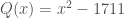
Example 1. Let’s factor the integer $N=2041$ . If we wanted to apply Fermat’s Factorization Method (factorization using differences of squares), we’d consider the values of $Q(x) = x^2-N$ , starting at $x = \lceil \sqrt{N} \rceil = 46$ , and look for squares. We produce the list

$75,\, 168, \, 263,\, 360, \, 459,\, 560, \, 663,\, 768,\, 875,\,\ldots$

These are quadratic residues (by construction), but none of these are squares, so Fermat would keep on looking. But what Kraitchik observes is that some of these outputs factor entirely into small primes:

$Q(46) = 75 = 3 \cdot 5^2,\,\, \quad Q(47) = 168 = 2^3 \cdot 3 \cdot 7,$

$Q(49) =360 = 2^3 \cdot 3^2 \cdot 5 , \,\,\quad Q(51) = 560= 2^4 \cdot 5 \cdot 7,$

$Q(53) = 768 = 2^8 \cdot 3, \,\,\quad Q(54) = 875 = 5^3 \cdot 7.$

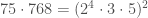
By looking at prime factorizations, it’s not hard to find a combination of these outputs that gives a perfect square. For example, $75 \cdot 768 = (2^4 \cdot 3 \cdot 5)^2$ . (There are a few others, too.) But, let’s not forget that these numbers came from values of $x^2 -N$ . In this example, we used the $x$ -values $46$ and $53$ . Thus

$(46 \cdot 53)^2 \equiv 46^2 \cdot 53^2 \equiv Q(46) \cdot Q(53) \equiv 75 \cdot 768 \equiv 240^2 \!\! \mod N.$

Since $46\cdot 53 \equiv 397 \!\! \mod N$ , this implies $397^2 \equiv 240^2 \!\! \mod N$ . Then $N \mid (397-240)(397+240)$ , and by computing

$\gcd(N, 397-240) = \gcd(2041, 157) = 157$

we get a non-trivial factor of $N$ . The full factorization is $N=2041 = 13 \cdot 157$ . //

The purpose of this article isn’t to rehash A Tale of Two Sieves. Rather, I’d like to explore the bits and pieces that make Pomerance’s example work so nicely. For contrast, here’s a bad example:

Example 2. Let’s factor $N= 1711$ . We define $Q(x) = x^2 -1711$ and compute $Q(42)=53$ , $Q(43) = 2 \cdot 3 \cdot 23$ , and $Q(44) = 3^2 \cdot 5^2$ . We thus produce a prime, a number with the ungainly factor $23$ , and a perfect square. In this case, Kraitchik’s Method reduces to the method of Fermat. It would have been easier to compute $1711 = 44^2 - 15^2 = (44-15)(44+15) = 29 \cdot 59$ . //

But that’s not the only way things can go wrong. Here’s a failure of a different sort:

Example 3. Let’s factor $N=767$ . We define $Q(x) = x^2 - 767$ and compute values of $Q(x)$ starting at $x = 28$ . In line with Pomerance’s $N=2041$ example, we want to focus on $x$ -values for which $Q(x)$ admits no prime factors larger than a given bound $B$ ; such integers are called $B$ -smooth. To stay specific, let’s choose $B=15$ here. The smallest value we test for smoothness is $Q(28) = 17$ ; after this, we compute $Q(29) = 2 \cdot 37$ , $Q(30) = 7 \cdot 19$ , and so forth. Each has a prime factor larger than $B=15$ , so we choose to discard them all.

Around now, the numbers start getting large. For the sake of efficiency, we might stop factoring $Q(x)$ completely. Instead, since we’re looking for $B$ -smooth outputs, we can perform trial division by small primes and give up if $Q(x)$ seems to misbehave. But herein lies the problem: if we cut off trial division at $B=15$ , say, we’d miss out on $Q(36) = 23^2$ and keep on going long after Fermat’s Factorization Method terminates.

This spirals. Searching even two million $Q(x)$ values turns up none which are $15$ -smooth. Are there tricks we could use to salvage this problem? Of course. We could increase the smoothness bound. We could switch to looking at $x^2 -2 N$ when the values of $Q(x)$ become too large. Still, these are things we’d hate to have to do when presenting an early example. //

Given all this, just how special is Pomerance’s example $N=2041$ ? Is it misleadingly (or in some sense even optimally) nice, or is it just one of many reasonable $N$ to consider? To answer this, let’s fix some properties that a “nice” introductory example should have:

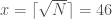
$N$ should have no factors less than $13$ . I’ll be the first to admit that the bound $13$ is somewhat arbitrary, but $N=2041$ passes this test (barely) and we certainly want to exclude integers which fall too easily to trial division. (At the bare minimum, things get strange if $N$ is even.)
$N$ should be a semiprime. This goes hand in hand with (1), since any number with three distinct prime factors of size at least $13$ already exceeds $4199$ . Moreover, it seems natural to look at semiprimes because one of the main “industrial applications” of factoring is the breaking of RSA keys.
The example shouldn’t devolve into Fermat’s Method. Factorization based on congruences of squares is often pitched as an improvement to Fermat’s Method. It’s therefore silly to work through an example that reverts back to this simpler technique. (See Example 2.)
The example shouldn’t require an overly large smoothness bound. Here, large is a bit subjective. Pomerance notes that the optimal smoothness bound for large $N$ is
$\displaystyle B \approx \mathrm{exp}\Big(\sqrt{\tfrac{1}{8} \log N \log\log N}\Big).$

Being charitable, we’ll call an example “bad” if the values of $Q(x)$ appear to escape to infinity before a square-producing subset of $5B$ -smooth numbers is found, where $B$ is as above.

These conditions create a fairly sparse of potential $N$ . Pomerance’s example $N=2041$ remains in the list, as do $36$ smaller examples:

$481, 793, 871, 949, 1079, 1207, 1219,1241,$
$1261,1313,1339,1349, 1357,1391,1411,1417,$
$1469,1501,1513,1577,1633,1649,1651,1679,$
$1717,1751,1781,1807,1817,1819, 1843,1909,$
$1921,1937,1963,2033$

Example 4. Let’s factor $N=481$ using Kraitchik’s Method. We form $Q(x) = x^2 -N$ and compute $Q(22) = 3$ and $Q(23) = 48 = 2^4 \cdot 3$ . Then $(22 \cdot 23)^2 \equiv (2^2 \cdot 3) ^2 \equiv 12^2 \!\! \mod 481$ . The computation

$\gcd(481, 22 \cdot 23 - 12) = 13$

gives a non-trivial factor of $N$ . //

I suppose the funny thing about this example is that it has succeeded a bit too well. To better highlight Kraitchik’s Method, let’s also restrict to the cases where first two outputs of $Q(x)$ don’t multiply to a perfect square. This eliminates $N=481$ and $N=949$ ; overall, only a slight change.

Example 5. Let’s factor $N=793$ using Kraitchik’s Method. As before, we form $Q(x) = x^2 - N$ and compute:

$Q(29) = 48 = 2^4 \cdot 3 \hspace{10 mm}\,$
$Q(30) = 107 \quad (\text{insufficiently smooth})$
$Q(31) = 168 = 2^3 \cdot 3 \cdot 7$
$Q(32) = 231 = 3 \cdot 7 \cdot 11$
$Q(33) = 296 \quad (\text{insufficiently smooth})$
$Q(34) = 363 = 3 \cdot 11^2.$

Then $(29 \cdot 34)^2 \equiv (2^2 \cdot 3 \cdot 11)^2 \!\! \mod N$ , and a GCD computation gives the non-trivial factor $61$ of $N$ . //

This is the first of our examples that feels like a solid introduction to Kraitchik’s Method. We have some smooth outputs, some not-so-smooth outputs, and enough terms to get you thinking about how you might find a square-producing subset in a more general case.

Pomerance does a few other computations with $N=2041$ which may explain his particular choice. It demonstrates, for example, that the first subset of quadratic residues which produces a perfect square might require more than two terms. The $N=2041$ case requires four terms: $75$ , $168$ , $360$ , and $560$ , although relations with fewer terms appear if one continues the computation.

If one wants to arrange for the first square-producing subset to use more than two terms, the list of admissible $N$ shrinks further. The full list of the $38$ such $N \leq 3000$ is given below:

$1079,1241,1261,1339,1391,1411,1469,1513,$
$1577,1633,1679,1717,1751,1807,1819,1843,$
$1921,1963,2041,2059,2119,2171,2227,2249,$
$2329, 2369,2413,2461,2489,2533,2561,2567,$
$2599,2641,2759,2831,2839,2951.$

Example 6. Let’s factor $N=1079$ using Kraitchik’s Method. As always, we form $Q(x) = x^2 - N$ and compute some values of $Q(x)$ . In this case, quite a few are insufficiently smooth. The useful ones are as follows:

$Q(33) = 10 = 2 \cdot 5, \quad Q(34) = 77 = 7 \cdot 11,$

$Q(39) = 2 \cdot 13 \cdot 17, \quad Q(43) = 770 = 2 \cdot 5 \cdot 7 \cdot 11.$

In this case, the first congruence of squares we find is not useful: it reads $770^2 \equiv 770^2 \!\! \mod 1079$ . We’d need to keep going. Unfortunately, the next smooth value we find is $Q(48) = 35^2$ , so this example (secretly) devolves into Fermat’s Method.

Example 7. Let’s factor $N=1241$ using Kraitchik’s Method. As always, we form $Q(x) = x^2 - N$ and compute some values of $Q(x)$ . Omitting the insufficiently smooth ones, we consider

$Q(36) = 55 = 5 \cdot 11, \quad Q(37) = 128 = 2^7,$

$Q(39) = 280 = 2^3 \cdot 5 \cdot 7, \quad Q(41) = 440 = 2^3 \cdot 5 \cdot 11.$

Then $(36 \cdot 37 \cdot 41)^2 \equiv (2^5 \cdot 5 \cdot 11)^2 \!\! \mod N$ , which is enough to find the non-trivial factor $73$ of $N$ . At long last, we’ve produced a truly beautiful example. //

In the previous example, we defined “sufficiently smooth” as $18$ -smooth. We are, after all, being five times more lenient in our definition of smooth than what is asymptotically optimal. Tightening this bound from $5B$ to $2B$ disqualifies $N=1241$ and makes $N=1261$ the new minimal example:

Example 8. Let’s factor $N=1261$ using Kraitchik’s Method. As always, we form $Q(x) = x^2 - N$ and compute some values of $Q(x)$ . Omitting the insufficiently smooth ones, we consider

$Q(36) = 35 = 5 \cdot 7, \quad Q(37) = 108 = 2^2 \cdot 3^3, \quad Q(41) = 420 = 2^2 \cdot 3 \cdot 5 \cdot 7.$

Then $(36 \cdot 37 \cdot 41)^2 \equiv (2^2 \cdot 3^2 \cdot 5 \cdot 7)^2 \!\! \mod N$ and we produce the non-trivial factor $13$ of $N$ . This examples matches $N=1241$ in complexity but requires less trial division to perform. //

As a parting gift, here’s a full list of $N \leq 10000$ which are admissible under our many conditions and the stricter smoothness bound $2B$ :

$1261, 1339, 1513, 1633, 1921, 2041, 2329, 2489,$
$2599, 2641, 2839, 2977, 3151, 3601,3679, 3781,$
$3809, 3841, 3991, 4061, 4321, 4369, 4531, 4579,$
$4681, 5149, 5161, 5287, 5371, 5377, 5833, 5921,$
$6001, 6157, 6289, 6511, 6799, 7009, 7141, 7201,$
$7291, 7409,7501, 7891, 7939, 7969, 8143, 8257,$
$8359, 8801, 8857, 9193, 9529, 9841, 9913, 9979.$

This list contains Pomerance’s example $N=2041$ and $55$ others. I imagine that most, if not all, would be fine “first examples” in the study of Kraitchik’s Method. (Although I have not verified that they avoid the pitfalls of Example 6.)

a. w. walker

mathematics and miscellany

Instructive Examples in Kraitchik’s Method

Leave a Reply Cancel reply

Share this:

Like this:

Leave a Reply Cancel reply