A Proof of Stirling’s Approximation via Contour Integration

A magnitude-argument plot of the gamma function.

Stirling’s approximation is a useful approximation for large factorials which states that the $n$ th factorial is well-approximated by the formula

$\displaystyle n! \sim (2\pi)^{\frac{1}{2}} n^{n+\frac{1}{2}} e^{-n}$

as $n \to \infty$ . Stirling’s approximation was first proven within correspondence between Abraham de Moivre and James Stirling in the 1720s; de Moivre derived everything but the leading constant, which Stirling eventually supplied (without proof; it’s not known how Stirling guessed it).

Given the rapid growth of the factorial, it is often more convenient to take logarithms and work with those instead. Doing so, Stirling’s approximation assumes the form

$\displaystyle\log n! = n \log n - n + \tfrac{1}{2} \log n + \tfrac{1}{2} \log(2\pi) + o(1).$

Most proofs of Stirling’s approximation work with the formulation above. One typical (modern-ish) proof begins by studying the integral approximation

$\displaystyle\log n! = \sum_{j =1}^n \log j = \int_1^n \!\Big(\log t +O(t^{-1})\Big) dt = n \log n - n + O(\log n).$

This version (as written) is too imprecise to recover Stirling’s Approximation, but the error term can be improved massively by introducing more terms using the Euler–Maclaurin formula (ca. 1735). This is the proof sketched on Wikipedia, for example.

The precise statement of the Euler–Maclaurin formula makes reference to the Bernoulli numbers $\{B_{2k}\}$ . These show up all over combinatorics, but as a multiplicative number theorist I will always think about Bernoulli numbers in the context of the Riemann zeta function. Specifically, one has $B_{2k} = -2k \zeta(1-2k)$ , so the Bernoulli numbers relate to special values of the zeta function.

This point of view inspired me to derive Stirling’s approximation (and the additional terms making up Stirling’s series) in a way which makes the role of the zeta function obvious. For convenience, we’ll phrase everything in terms of the gamma function; this affects the shape of our formula in a small and readily-understandable way. Without further ado, here’s the proof:

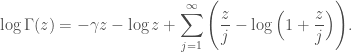
Proof: We begin with Weierstrass’ infinite product for the gamma function (ca. 1854),

$\displaystyle\Gamma(z) = e^{-\gamma z} z^{-1} \prod_{j=1}^\infty \frac{e^{z/j}}{1+z/j},$

in which $\gamma$ is the Euler–Mascheroni constant. (Euler gave an infinite product for the gamma function back in 1729 which might also work for this proof technique.) Taking a principal branch of the logarithm, we produce

$\displaystyle\log \Gamma(z) = - \gamma z - \log z + \sum_{j=1}^\infty \Bigg( \frac{z}{j} - \log\Big(1+\frac{z}{j}\Big) \Bigg).$

Our next ingredient is a contour integral representation of the logarithm; namely,

$\displaystyle\log(1+z) = \frac{1}{2\pi i} \int_{(\frac{1}{2})} \frac{\pi \csc(\pi s)}{s} z^s \, ds,$

in which the line of integration is the vertical line with real part $\frac{1}{2}$ . This formula can be proven by Cauchy’s residue formula (and analytic continuation in $z$ ). We note as well an interpretation via Mellin transforms: this formula states that the Mellin transform of $\log(1+z)$ is $\pi \csc(\pi s)/s$ . (See here for a table listing this and other Mellin pairs.)

In any case, by combining our formulas and shifting the contour to the right, we produce

$\displaystyle\log \Gamma(z) = - \gamma z - \log z + \sum_{j =1}^\infty \Bigg( \frac{z}{j} - \frac{1}{2\pi i} \int_{(\frac{1}{2})} \frac{\pi \csc(\pi s)}{s} \bigg(\frac{z}{j}\bigg)^s \, ds\Bigg)$

$=\displaystyle -\gamma z - \log z - \sum_{j=1}^\infty \frac{1}{2\pi i} \int_{(\frac{3}{2})} \frac{\pi \csc(\pi s)}{s} \bigg(\frac{z}{j}\bigg)^s \, ds.$

Absolute convergence of the contour integral justifies an interchange of sum and integral and allows us to recognize a zeta function:

$\displaystyle \log \Gamma(z) = -\gamma z - \log z - \frac{1}{2\pi i} \int_{(\frac{3}{2})}\frac{\pi \csc(\pi s)}{s} \sum_{j=1}^\infty\bigg(\frac{z}{j}\bigg)^s \, ds$

$\displaystyle =-\gamma z - \log z - \frac{1}{2\pi i} \int_{(\frac{3}{2})} \frac{\pi \csc(\pi s)}{s} z^s \zeta(s)\, ds.$

We can now shift the contour of integration back to the left, extracting residues as we go. The residue from the double pole at $s=1$ is $z-\gamma z - z\log z$ , hence

$\displaystyle \log \Gamma(z) =z \log z -z - \log z -\frac{1}{2\pi i} \int_{(\frac{1}{2})} \frac{\pi \csc(\pi s)}{s} z^s \zeta(s)\, ds.$

(From here on out, we identify the Riemann zeta function with its meromorphic continuation.) Shifting farther left passes a second double pole at $s=0$ , which has residue $-\frac{1}{2}\log z - \frac{1}{2} \log(2\pi)$ , hence

$\displaystyle\log \Gamma(z) = z \log z - z +\tfrac{1}{2} \log z + \tfrac{1}{2} \log(2\pi) - \frac{1}{2\pi i} \int_{(-\frac{1}{2})}\!\!\! \frac{\pi \csc(\pi s)}{s} z^s \zeta(s) ds.$

A bound in absolute value shows that the integral at right in the line above is $o(1)$ and therefore small enough to recover Stirling’s approximation. $\square$

With the proof complete, I offer two final remarks:

1. There’s nothing stopping us from shifting the line of integration in our formula even farther left. Doing so passes simple poles at the negative odd integers, which we can extract as residue terms in our formula. (The poles at negative even integers are cancelled by trivial zeros of the zeta function.) This yields

$\displaystyle\log \Gamma(z) = z \log z - z + \tfrac{1}{2} \log z + \tfrac{1}{2}\log(2\pi)$

$\displaystyle + \sum_{n=1}^N \frac{\zeta(1-2n)}{1-2n} z^{1-2n} + O\Big(z^{-2N}\Big),$

which is equivalent to Stirling’s series.

2. In one of Keith Conrad’s online notes, he subdivides proofs of Stirling’s approximation according to the origin of the mysterious factor $\sqrt{2\pi}$ . Conrad lists references in which $\pi$ is obtained through (a) infinite products (such as the Wallis product), (b) the Gaussian integral, and (c) reflection formulas for the gamma function. In the proof we give here, we obtain $\sqrt{2\pi}$ from the series expansion

$\zeta(s) = - \tfrac{1}{2} - \tfrac{1}{2} \log(2\pi) s + O(s^2)$

in the limit as $s\to 0$ . Because the functional equation of zeta invokes gamma functions, you could argue that this proofs falls in camp (c). However, the proof here is quite different from that given in the Conrad’s example for (c) (which was taken from section 5.2.5 in Ahlfors’ book Complex Analysis). Both proofs begin with the Weierstrass product, but their use of contour integration is quite different. The proof given here is also shorter.

One response to “A Proof of Stirling’s Approximation via Contour Integration”

Jean S October 19, 2021 at 12:52 am · · Reply →

I enjoyed readding this

LikeLike

a. w. walker

mathematics and miscellany

A Proof of Stirling’s Approximation via Contour Integration

One response to “A Proof of Stirling’s Approximation via Contour Integration”

Leave a Reply Cancel reply

Share this:

Like this:

One response to “A Proof of Stirling’s Approximation via Contour Integration”

Leave a Reply Cancel reply