Quadratic Reciprocity and the Theta Function

*Argument plot of the classical Jacobi theta function.*

The law of quadratic reciprocity is a beautiful result in elementary number theory which relates the Legendre symbols $(\frac{p}{q})$ and $(\frac{q}{p})$ . For $p$ and $q$ odd primes, it states that

$\displaystyle \Big(\frac{p}{q}\Big)\Big(\frac{q}{p}\Big) = \begin{cases}1, \quad & p \text{ or } q \equiv 1 \bmod 4, \\ -1, \quad & p \text{ and } q \equiv 3 \bmod 4. \end{cases}$

One of the better-known proofs of quadratic reciprocity involves the quadratic Gauss sum, an exponential sum defined by

$\displaystyle g_p := \sum_{a=1}^p \Big(\frac{a}{p}\Big) e\Big(\frac{a}{p}\Big),$

in which $e(x) := e^{2\pi i x}$ . In essence, this proof works by computing $g_p^q$ in two ways:

Euler’s criterion: $g_p^q \equiv g_p \cdot (g_p^2)^{\frac{q-1}{2}} \equiv g_p \cdot (\frac{g_p^2}{q}) \bmod q$ . Note that this is well-defined because $p^* := g_p^2 = (\frac{-1}{p}) p$ is an integer.
Fermat’s Little Theorem (for algebraic integers): Working in the cyclotomic field $\mathbb{Q}(\zeta_p)$ , we find that $g_p^q \equiv \sum_{a(p)} (\frac{a}{p}) e(\frac{aq}{p}) \bmod q$ . Changing variables $a \mapsto q^{-1} a \bmod p$ gives $g_p^q \equiv (\frac{q}{p}) g_p \bmod q$ .

It follows that $(\frac{p^*}{q}) \equiv (\frac{q}{p}) \bmod q$ , which implies quadratic reciprocity.

In this note, we give a second proof of quadratic reciprocity using the analytic properties of the Jacobi theta function $\theta(z)$ , which is a modular form of weight $\frac{1}{2}$ . In particular, we produce two formulas for the behavior of $\theta(z)$ as $z \to p/q$ , and derive quadratic reciprocity by comparing them. As in the previous proof, Gauss sums play a prominent role. Otherwise, this proof is distinct; in particular, it avoids Euler’s criterion and any semblance of algebraic number theory.

— THE JACOBI THETA FUNCTION —

The Jacobi theta function $\theta(z)$ is defined on the upper half-plane by the series $\theta(z) = \sum_{n \in \mathbb{Z}} e(n^2 z)$ . It is a modular form of weight $\frac{1}{2}$ on the congruence subgroup $\Gamma_0(4)$ , transforming via

$\displaystyle \theta(\gamma z) = j_\theta(\gamma, z) \theta(z) = \epsilon_d^{-1} \Big(\frac{c}{d}\Big) (cz+d)^{\frac{1}{2}} \theta(z), \quad \gamma = \Big( \begin{matrix} a & b \\ c & d \end {matrix} \Big) \in \Gamma_0(4),$

in which $\epsilon_d = 1$ for $d \equiv 1 \bmod 4$ , $\epsilon_d =i$ for $d \equiv 3 \bmod 4$ , and $(\frac{c}{d})$ denotes Kronecker’s extension of the Legendre symbol. In addition, $\theta(z)$ satisfies the functional equation $\theta(-1/4z) = (-2iz)^{1/2} \theta(z)$ , which follows from Poisson summation and analytic continuation. (In both functional equations, we use the principal square root on $\mathbb{C}$ .)

We only need the second functional equation in our proof, but we will use it several times. For starters, it implies that $\theta(iy) \sim (2y)^{-1/2}$ as $y \to 0$ from above. And more generally, this asymptotic implies that

$\displaystyle \sum_{n \equiv a (p)} e^{-2\pi n^2 y} \sim \frac{1}{p} \cdot (2y)^{-\frac{1}{2}}$

as $y \to 0$ , for any choice of $a \bmod p$ . (Hint: Use the squeeze theorem to compare the asymptotics with different choices of $a$ .)

— THE BEGINNING OF A PROOF —

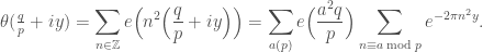
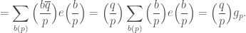
We now begin our proof in earnest. Let $p$ and $q$ be odd primes, and consider the limit of $\theta(\frac{q}{p} + iy)$ as $y \to 0$ . We have

$\displaystyle \theta(\tfrac{q}{p}+iy) = \sum_{n \in \mathbb{Z}} e\Big(n^2\Big(\frac{q}{p}+iy\Big)\Big) = \sum_{a (p)} e\Big(\frac{a^2 q}{p} \Big) \sum_{n \equiv a \bmod p} e^{-2\pi n^2 y}.$

In the limit as $y \to 0$ , each inner sum grows as $p^{-1} (2 y)^{-1/2}$ . For the outer sum over $a \bmod p$ , we let $\overline{q}$ denote $q^{-1} \bmod p$ and observe that

$\displaystyle \sum_{a(p)} e\Big(\frac{a^2 q}{p} \Big) = \sum_{b(p)} \Big(1+ \Big(\frac{b}{p}\Big)\Big) e\Big(\frac{bq}{p}\Big) = \sum_{b(p)} \Big(\frac{b}{p}\Big) e\Big(\frac{bq}{p}\Big)$
$\displaystyle = \sum_{b(p)} \Big(\frac{b\overline{q}}{p}\Big) e\Big(\frac{b}{p}\Big) = \Big(\frac{q}{p}\Big) \sum_{b(p)} \Big(\frac{b}{p}\Big) e\Big(\frac{b}{p}\Big) = \Big(\frac{q}{p}\Big) g_p.$

It follows that $\theta(\tfrac{q}{p} + iy) \sim p^{-1} (2 y)^{-\frac{1}{2}} (\frac{q}{p}) g_p$ as $y \to 0$ . We will use this asymptotic a few times in what follows.

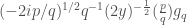
From the functional equation $\theta(-1/4z) = (-2iz)^{1/2} \theta(z)$ , we see that

$\displaystyle \theta\Big(\frac{-1}{4(\frac{p}{q}+iy)}\Big) = (-2i (\tfrac{p}{q}+iy))^{\frac{1}{2}} \theta(\tfrac{p}{q}+iy).$

As $y \to 0$ , the right-hand side tends to $(-2ip/q)^{1/2} q^{-1} (2y)^{-\frac{1}{2}} (\frac{p}{q}) g_q$ . Meanwhile, the left-hand side equals $\theta(\frac{-q}{4p} + i \frac{q^2}{4p^2} y + O(y^2))$ . Ignoring the non-dominant $O(y^2)$ term, this tends to

$\displaystyle \sum_{a(4p)} e\Big(\frac{-a^2 q}{4p}\Big) \cdot \frac{1}{4p} \Big(\frac{2q^2 y}{4p^2}\Big)^{-\frac{1}{2}} = (2 y)^{-\frac{1}{2}} \frac{1}{2q} \sum_{a(4p)} e\Big(\frac{-a^2 q}{4p}\Big).$

The sum over $a \bmod 4p$ is a generalized Gauss sum. By the Chinese remainder theorem, we have

$\displaystyle \sum_{a(4p)} e\Big(\frac{-a^2 q}{4p}\Big) = \sum_{a(p)} e\Big(\frac{-4a^2 q}{p}\Big) \sum_{a(4)} e\Big(\frac{-a^2 pq}{4}\Big).$

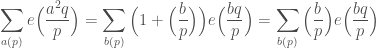
The first exponential sum is $(\frac{-4q}{p}) g_p = (\frac{-1}{p})(\frac{q}{p}) g_p$ . The second depends only on $pq \bmod 4$ and can be computed exactly; we see that it equals $2-2i$ when $pq \equiv 1 \bmod 4$ and $2+2i$ when $pq \equiv 3 \bmod 4$ . It follows that

$\displaystyle \theta\Big(\frac{-1}{4(\frac{p}{q}+iy)}\Big) = (2 y)^{-\frac{1}{2}} \frac{1}{2q} \Big(\frac{-1}{p} \Big)\Big(\frac{q}{p}\Big) g_p \cdot \begin{cases} 2-2i, \quad & pq \equiv 1 \bmod 4 \\ 2+2i, \quad & pq \equiv 3 \bmod 4 \end{cases}$

in the limit as $y \to 0$ .

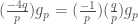
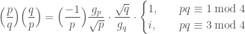
Of course, these two expressions for the limiting behavior must agree. After some simplification, we conclude that

$\displaystyle \Big(\frac{p}{q}\Big)\Big(\frac{q}{p}\Big) = \Big(\frac{-1}{p}\Big) \frac{g_p}{\sqrt{p}} \cdot \frac{\sqrt{q}}{g_q} \cdot \begin{cases} 1, \quad & pq \equiv 1 \bmod 4 \\ i, \quad & pq \equiv 3 \bmod 4 \end{cases}$

Note that the right-hand side has absolute value $1$ because $\vert g_p \vert = \sqrt{p}$ as a consequence of $g_p^2 = (\frac{-1}{p}) p$ , and the same for $q$ . (Note that the cases in the previous line could be written $\epsilon_{pq}$ .)

— THE SIGN OF THE GAUSS SUM —

Recall that the Gauss sum $g_p$ is one of the complex square roots of $(\frac{-1}{p}) p$ . At this point, we could prove quadratic reciprocity if we knew which square-root (depending on $p$ ) to choose. The correct choice of sign is of course well-known now, but it took Gauss a few years to determine the sign after first introducing the Gauss sums. Fortunately, we find ourselves in a position to determine the sign of $g_p$ immediately.

The key observation is that none of our formulas so far have required $p$ and $q$ to be odd primes. In fact, it is enough for $p$ and $q$ to be odd, coprime, and square-free. Taking $p$ prime and $q=1$ in the previous offset equation gives

$\displaystyle 1 = \Big(\frac{-1}{p}\Big) \frac{g_p}{\sqrt{p}} \epsilon_p \quad \Longrightarrow \quad g_p = \epsilon_p^{-1} \Big(\frac{-1}{p}\Big) \sqrt{p} = \epsilon_p \sqrt{p}.$

Of course, $g_q = \epsilon_q \sqrt{q}$ as well. Returning to the same offset equation from before, it follows that

$\displaystyle \Big(\frac{p}{q}\Big)\Big(\frac{q}{p}\Big) = \frac{\epsilon_{pq}}{\epsilon_p \epsilon_q}.$

The right-hand side only depends on the values of $p$ and $q$ mod $4$ . And, as expected, it equals $1$ unless both $p \equiv 3 \bmod 4$ and $q \equiv 3 \bmod 4$ , when it equals $-1$ . This completes our proof of quadratic reciprocity.