Notes on the Chebyshev Theorem

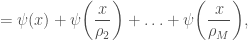
In 1737, Euler presented a novel proof of the infinitude of the primes, in showing that the harmonic sum of the primes diverges. Explicitly, Euler’s work furnishes the estimate

$\displaystyle\sum_{p \leq x} 1/p=\log \log x + O(1),$

in which the sum exhausts the rational primes at most $x$ . At this point, it becomes quite elementary to derive the two inequalities

$\displaystyle\limsup_{n \to \infty} \frac{p_n}{n \log n} \geq 1 \quad \text{and} \quad \liminf_{n \to \infty} \frac{p_n}{n \log n} \leq 1.$

Results of this flavor remained essentially unimproved for over a century, until Chebyshev presented the following landmark theorem in 1852:

Theorem (Chebyshev): There exist positive constants $c_1,c_2$ such that

$\displaystyle c_1 \leq \liminf_{x \to \infty} \frac{\pi(x)\log x}{x} \leq \limsup_{x \to \infty} \frac{\pi(x) \log x}{x} \leq c_2.$

Thus Chebyshev’s Theorem shows that $x/\log x$ represents the growth rate (up to constants) of $\pi(x)$ ; stated equivalently in Bachmann-Landau notation, we have $\pi(x) \in \Theta(x/\log x)$ . Yet more is true: the constants $c_1,c_2>0$ in Chebyshev’s proof are therein made effective, and can be taken as

$c_1 =\frac{\log 2}{2} +\frac{\log 3}{3} + \frac{\log 5}{5}-\frac{\log 30}{30} \approx 0.921292;$

$c_2 = \frac{6}{5}\left(\frac{\log 2}{2} +\frac{\log 3}{3} + \frac{\log 5}{5}-\frac{\log 30}{30}\right)\approx1.10555.$

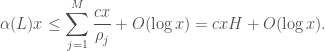
As a corollary to Chebyshev’s Theorem, we have $\pi(2n-3)>\pi(n)$ for $n \gg 0$ . By making this implicit bound on $n$ precise, Chebyshev was able to prove Bertrand’s Postulate (thereafter known as the Bertrand-Chebyshev Theorem).

In this post we’ll prove a variant of Chebyshev’s Theorem in great generality, and discuss some historically competitive bounds on the constants $c_1$ and $c_2$ given above. Lastly, we’ll discuss how Chebyshev’s Theorem relates to proposed “elementary” proofs of the PNT.

— PART I (LEMMAS) —

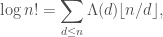
To begin, let $\Lambda(n)$ denote the von Mangoldt function, and let $\psi(n)$ denote the second Chebyshev function

$\displaystyle\psi(n):=\sum_{d \leq n} \Lambda(n) = \sum_{p^k \leq n} \log p.$

We recall that $\psi(x) \sim \pi(x) \log x$ (by elementary methods), whereby it suffices in the context of Chebyshev’s Theorem to study the asymptotic growth of $\psi(x)$ . This (given the complexity of the PNT) is understandably difficult, and so our first step towards Chebyshev’s result is to approximate $\psi$ by “simpler” functions.

For what follows, let $L=\{\ell_1,\ldots, \ell_k\}$ be a multi-set of non-zero integers. We define the two functions

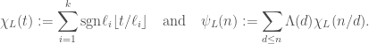
$\displaystyle\chi_L(t):=\sum_{i=1}^k \mathrm{sgn} \ell_i \lfloor t/\ell_i \rfloor \quad \text{and} \quad \psi_L(n) :=\sum_{d \leq n} \Lambda(d) \chi_L(n/d).$

If $\sum_L 1/\ell =0$ , we’ll say that $L$ is balanced. In this case, the following Lemma provides the asymptotic growth of $\psi_L$ :

Lemma 1: If $L$ is balanced, then

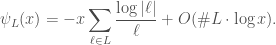
$\displaystyle\psi_L(x)= -x \sum_{\ell \in L} \frac{\log \vert \ell\vert}{\ell} +O(\# L \cdot\log x).$

Proof: To begin, consider the identity

$\log n! = \displaystyle\sum_{d \leq n} \Lambda(d) \lfloor n/d \rfloor,$

which expresses Legendre’s formula (1808) in terms of the von Mangoldt function. Extending by linearity, we obtain

$\displaystyle \sum_L \mathrm{sgn} \ell \log (n/\vert \ell \vert)! = \sum_L \mathrm{sgn} \ell \sum_{d \leq n} \Lambda(d) \left\lfloor \frac{n}{d \vert \ell \vert} \right\rfloor = \sum_{d \leq n} \Lambda(d) \chi_L(n/d),$

i.e. an expression of $\psi_L(n)$ as the logarithm of a ratio of factorials. To continue, we now recall Stirling’s approximation (in its weak form), that $\log n! = n \log n - n +O(\log n)$ . Accordingly, we obtain

$\psi_L(n) =\displaystyle\sum_L \mathrm{sgn} \ell \left(\frac{n}{\vert \ell \vert} \log (n/\vert \ell \vert) -\frac{n}{\vert \ell \vert} \right) +O(\# L \cdot \log n)$

$=\displaystyle\sum_L\frac{n}{\ell}\log n-\sum_L \frac{n}{\ell} \log \vert \ell \vert - \sum_L \frac{n}{\ell}+O(\# L \cdot \log n).$

As $L$ is balanced, the first and third sums vanish and our result follows. $\square$

(Note: In the proof of Lemma 1 we remarked that $\psi_L$ arises as the logarithm of a ratio of factorials. On the other hand, 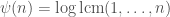$\psi(n) = \log \mathrm{lcm}(1,\ldots,n)$ , and we may view our general technique as an estimation of $\mathrm{lcm}(1,\ldots,n)$ as a ratio of factorials.)

For future use, we define 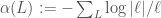$\alpha(L):= -\sum_L \log \vert \ell\vert/\ell$ .

With Lemma 1 in hand, we seek to relate the growth of $\psi$ and $\psi_L$ . To do so, we first note that $\chi_L$ is periodic (with period dividing $\mathrm{lcm}(L)$ ), provided that $L$ is balanced. In particular, $\chi_L$ is bounded; let $M$ (resp. $m$ ) denote the maximum (resp. minimum) of $\chi_L$ . Define $\eta_j = \min \{n \geq 1 : \chi_L(n) \leq -j\}$ , if such an $\eta_j$ exists (i.e. for $j \leq \vert m \vert$ ). Lemma 2 gives an upper bound for $\psi$ :

Lemma 2: Let $L$ be balanced, and suppose that $h:=\sum_{j=0}^{\vert m \vert} 1/\eta_j <1$ . Then

$\displaystyle \limsup_{x \to \infty} \frac{\psi(x)}{x} \leq \frac{\alpha(L)}{1-h}.$

Proof: By definition of $\eta_j$ , we have $\chi_L(x/d) \geq j+1$ for $d \in (x/\eta_j,x]$ . As $\Lambda \geq 0$ , it follows that

$\psi_L(x) \displaystyle\geq \sum_{d \in (\frac{x}{\eta_0},x]}\Lambda(d) +\sum_{d \in (\frac{x}{\eta_2},\frac{x}{\eta_1}]} -\Lambda(d) + \ldots + \sum_{d \leq x/\eta_{\vert m \vert}} m \Lambda(d)$

$=\displaystyle\psi(x)-\psi\bigg(\frac{x}{\eta_0}\bigg)-\!\sum_{j=0}^{\vert m \vert-1}\! j\bigg(\psi\bigg(\frac{x}{\eta_{j}}\bigg)\!-\!\psi\bigg(\frac{x}{\eta_{j+1}}\bigg)\bigg)\!+\!m\psi\bigg(\frac{x}{\eta_{\vert m \vert}}\bigg).$

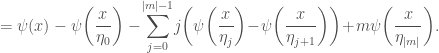
This last expression telescopes, and we obtain (after iterated substitution)

$\displaystyle\psi(x) \leq \psi_L(x) + \sum_{j=0}^{\vert m \vert} \psi(x/\eta_j)\leq\!\!\!\!\!\! \sum_{(a_0,\ldots,a_{\vert m \vert}) \in A}\!\!\!\binom{\sum a_i}{a_0,\ldots,a_{\vert m\vert}}\psi_L\bigg(\!\frac{x}{\eta_0^{a_0} \cdots \eta_{\vert m \vert}^{a_{\vert m \vert}}}\!\bigg),$

in which $A$ denotes the cube $[0, \log_{\eta_0} x]^{\vert m \vert +1}$ and $\binom{\sum a_i}{a_0,\ldots,a_{\vert m \vert}}$ represents the multinomial coefficient. With Lemma 1, this implies

$\displaystyle \psi(x) \leq \sum_A \binom{\sum a_i}{a_0,\ldots,a_{\vert m \vert}} \frac{\alpha(L)x}{\eta_0^{a_0} \cdots \eta_{\vert m \vert}^{a_{ \vert m \vert}}}+O((\log x)^{\vert m \vert +2}).$

Now, it follows from the multinomial theorem that

$\displaystyle \psi(x) \leq \alpha(L) x \sum_{j=0}^{\log_{\eta_0} x} h^j +O((\log x)^{\vert m \vert +2}) \leq \frac{\alpha(L)x}{1-h}+O((\log x)^{\vert m \vert +2}),$

and this proves Lemma 2. $\square$

In our final lemma, we derive a lower bound for $\liminf \psi(x)/x$ . Recall that $\chi_L$ is bounded (with maximum $M$ dependent on $L$ ) provided that $L$ is balanced. For $j \leq M$ , we define $\rho_j:= \min\{n \geq 1 : \chi_L(n) \geq 1\}$ , and then set 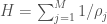$H = \sum_{j=1}^M 1/\rho_j$ . We then have:

Lemma 3: Let $L$ be balanced, and suppose that $\rho_1=1$ . Then

$\displaystyle\liminf_{x \to \infty} \frac{\psi(x)}{x} \geq \frac{\alpha(L)}{H}.$

Proof: By definition of $\rho_j$ (and our hypothesis on $\rho_1$ ), we have

$\displaystyle\psi_L(x) \leq \!\!\sum_{d \in (\frac{x}{\rho_2},x]}\!\! \Lambda(d) + \!\!\sum_{d \in (\frac{x}{\rho_3},\frac{x}{\rho_2}]}\!\! 2 \Lambda(d)+ \ldots + \!\!\sum_{d \leq x/\rho_M}\!\! M \Lambda(d)$

$=\displaystyle\psi(x)+ \psi\bigg(\frac{x}{\rho_2}\bigg)+\ldots+\psi\bigg(\frac{x}{\rho_M}\bigg),\quad$

as the previous expression telescopes. Let $c \in \mathbb{R}$ be a lower bound for $\psi(x)/x$ as $x \to \infty$ (these lower bounds exist by positivity of $\psi$ ). Then $\psi(x/\rho_j) \leq c x/\rho_j$ for large $x$ , and thus

$\alpha(L)x \leq \displaystyle\sum_{j=1}^M \frac{cx}{\rho_j} + O(\log x)=cxH+O(\log x).$

In particular, this forces $\alpha(L)/H \leq c$ for all lower bounds $c$ ; Lemma 3 follows in passing to the liminf. $\square$

— PART II —

Now, we present some applications of the lemmas in Part I. Our first example concerns the simplest of all balanced multi-sets:

Example 1: In this example, we take $L=\{1,-2,-2\}$ . Then $\chi_L$ satisfies

$\chi_L(t) = \begin{cases} 0, \quad \text{if } \lfloor t \rfloor \equiv 0 \mod 2 \\ 1, \quad \text{if } \lfloor t \rfloor \equiv 1 \mod 2;\end{cases}$

in particular, $M =1$ (with $\rho_1 =1$ ), and $m=0$ (with $\eta_0 =2$ ). Noting that $\alpha(L)=\log 2$ , we conclude (via Lemmas 2-3) that

$\displaystyle 0.693147 \approx \log 2 \leq \liminf_{x \to \infty}\frac{\psi(x)}{x} \leq \limsup_{x \to \infty} \frac{\psi(x)}{x} \leq 2 \log 2 \approx 1.38629.$

The relationship between $\psi_L$ and the central binomial coefficients (cf. Lemma 1) is far from coincidental: a more-precise study of these coefficients yields a proof of Bertrand’s Postulate (an observation due to Erdős). Yet this is likely the extent to which the central binomial coefficients encapsulate the density of primes, as the upper and lower bounds on $\psi$ differ here by a factor of two (cf. $\pi((2+\epsilon)n)\gg\pi(n)$ for all $\epsilon>0$ ).

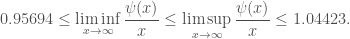
Example 2: Our second example comes from Chebyshev (1852), and is generated by the (balanced) multi-set $L=\{1,-2,-3,-5,30\}$ . We readily find $M=1$ (with $\rho_1 =1$ ) and $m=0$ (with $\eta_0 =6$ ), which yields the bounds

$\displaystyle 0.92129 \approx c_1 \leq \liminf_{x \to \infty}\frac{\psi(x)}{x} \leq \limsup_{x \to \infty} \frac{\psi(x)}{x} \leq c_2 \approx 1.10555$

(exact values for $c_1,c_2$ are given in the introduction). As remarked above, these bounds suffice to give an elementary proof of Bertrand’s Postulate, which may explain why Chebyshev makes no attempt to further improve them (at least, not in his original manuscript, Mémoire sur les nombres premiers).

On the other hand, it’s quite possible that Chebyshev could not find other multi-sets that improved upon these bounds. Indeed, insofar as required to prove Bertrand’s Postulate (for all $n$ , not just asymptotically), the multi-set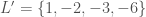 $L'=\{1,-2,-3,-6\}$ affords a similar — yet far shorter — proof.

The torch that Chebyshev lit was carried in subsequent decades by Sylvester, who in 1892 published the bounds

$\displaystyle 0.95694 \leq \liminf_{x \to \infty} \frac{\psi(x)}{x} \leq \limsup_{x \to \infty} \frac{\psi(x)}{x} \leq 1.04423.$

In a sense, these bounds were penultimate: within four years two proofs of the PNT were published (due to Hadamard and de la Vallée-Poussin).

Example 3: Now, to find for ourselves some competitive bounds on $\psi$ , we embrace that which Chebyshev could not: brute force search over short multi-sets $L$ . In a few hundred hours of CPU time (in Mathematica), I’ve found the following:

$L_1=\{1,-2,-3,-5,6,10,-11,-19,-36,-45,-57,-76,-110\}$

$L_2=\{1,-2,-3,-5,6,-7,10,-11,-13,$

$14,15,-17,-455,595,-715\},$

which induce the lower (resp. upper) bounds $0.95616$ and $1.05829$ on the infimum and supremum of $\psi(x)/x$ , respectively. Unfortunately, I have yet to find multi-sets that improve upon the elementary bounds of Sylvester (which — credit to him — require far more delicate approximations). Nevertheless, the lower bound which stems from $L_1$ lies within spitting distance ( $\approx 0.00078$ ) of Sylvester’s bound, a non-trivial feat in itself.

— PART III —

After 1896, the Chebyshev Theorem (and extensions thereof) became little more than a historical/pedagogical note. But the nagging question remains: could Chebyshev (in theory) have proven the PNT with this approach?

In short, maybe. Under the assumption of the PNT, three proofs emerged (circa 1937; due independently to Erdős, Kalmár, and Rosser) that showed that the constants in Chebyshev’s proof could be forced arbitrarily close to one. (Due to a miscommunication none saw publication until 1980, when Erdős and Diamond reconstructed a proof in the memory of Kalmár.)

I confess that the techniques presented hitherto in this article are too ad hoc to reach this result. That is, in building upon the weak foundation of Egyptian fractions to create multi-sets $L$ with desirable properties, we find ourselves limited by the unpredictability of Egyptian fraction representations.

Morally, then, our multi-sets $L$ form great examples but remain too unwieldy for use in a theoretic capacity. All the same, it takes only a small tweak of our previous methods to reach the result above, which we prove now as a fitting end to this article:

Proof: Consider the multi-set

$L=L_n:=\{1,-2,-3,\ldots, n\mu(n)\}.$

Then $L$ is not necessarily balanced. (In fact, Bertrand’s Postulate implies that $L$ is never balanced; see the Exercises.) Nevertheless, if we set $\sigma = -(n+1) \sum_{j=1}^n \mu(j)/j$ , the modified $\chi_L$ function

$\displaystyle\widehat{\chi}_L(t):= \bigg(\sum_L \mathrm{sgn} \ell \lfloor t/\vert \ell \vert \rfloor \bigg)+ \sigma \lfloor t/(n+1) \rfloor$

is periodic — with period dividing $\mathrm{lcm}(1,\ldots, n+1)$ — and is consequently bounded. Next, we introduce the “indicator function”

$\displaystyle\widehat{e}_L:= \sum_L \mathrm{sgn} \ell e_{\vert\ell \vert} + \sigma e_{n+1}=\sum_{j=1}^n \mu(j)e_j +\sigma e_{n+1},$

in which the arithmetic function $e_j(k) : \mathbb{N} \to \{0,1\}$ denotes the Kronecker Delta $\delta_{j,k}$ . For brevity, set $\widehat{g}_L:= 1 * \widehat{e}_L$ (as a Dirichlet convolution), which we note satisfies $\widehat{\chi}_L(x)=\sum_{n \leq x} \widehat{g}_L(n).$

Our proof now commences in earnest. With the convolution identity $\Lambda * 1 = \log$ (the so-called Chebyshev Identity), we derive

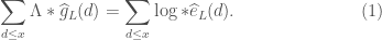
$\displaystyle\sum_{d \leq x} \Lambda * \widehat{g}_L(d) = \sum_{d \leq x} \log * \widehat{e}_L(d). \quad\qquad\qquad\qquad (1)$

The right-hand side of $(1)$ may be rewritten as

$\displaystyle\sum_{ij \leq x} \log i \,\widehat{e}_L(j) = \sum_{j \leq x} \bigg( \sum_{i \leq x/j} \log i \bigg) \widehat{e}_L(j)=\sum_{j \leq x} \log(x/j)! \widehat{e}_L(j).$

Using Stirling’s Approximation (just as in Lemma 1), we obtain the asymptotic

$\displaystyle \sum_{d \leq x} \log * \widehat{e}_L(d) = \widehat{\alpha}(L_n) + O(n \log x), \,\,\quad\qquad \qquad (2)$

in which $\widehat{\alpha}(L_n)$ denotes the constant

$\displaystyle-\bigg( \!\sum_{j=1}^n \frac{\mu(n) \log n}{n} + \frac{\sigma \log(n+1)}{n+1}\!\bigg)= \alpha(L_n)+ \log(n+1)\sum_{j=1}^n \frac{\mu(j)}{j}.$

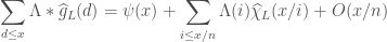
Now turning to the left-hand side of $(1)$ , an application of the Dirichlet Hyperbola method gives

$\displaystyle\sum_{ij \leq x} \Lambda(i) \widehat{g}_L(j)\!= \!\sum_{j \leq n} \psi(x/j) \widehat{g}_L(j)\!+\!\sum_{i \leq x/n} \Lambda(i) \widehat{\chi}_L(x/i)\!- \!\widehat{\chi}_L(n)\psi(x/n).$

By construction, $\widehat{\chi}_L=1$ on the interval $[1,n+1)$ . In particular, the rightmost term above is nothing more than $\psi(x/n)$ , which is $O(x/n)$ by our estimates in Part II. Moreover, since $\widehat{\chi}_L$ represents the summary function of $\widehat{g}_L$ , it follows that $\widehat{g}_L=e_1$ on $[1,n+1)$ . And so, the second sum in the line above simplifies to $\psi(x)$ , and we obtain at last:

$\displaystyle \sum_{d \leq x} \Lambda * \widehat{g}_L(d)=\psi(x)+\sum_{i \leq x/n} \Lambda(i) \widehat{\chi}_L(x/i)+O(x/n)$

$\sim \psi(x)+\widehat{\alpha}(L_n)x/n+O(n\log x)+O(x/n),$

wherein the final simplification comes from direct analogy with Lemma 1. Coupled with lines $(1)$ and $(2)$ , this implies

$\psi(x) = \widehat{\alpha}(L_n)(1-1/n)x+O(x/n)$

(provided that $n = o(\log x)$ for simplicity). For fixed $\epsilon >0$ , we obtain

$\psi(x) = (\widehat{\alpha}(L_n)-\epsilon)x+O(\epsilon x) \qquad\qquad\qquad \qquad (3)$

for all $n$ sufficiently large (e.g. $n>1/\epsilon$ ).

At this point in our proof, we need only show that $\widehat{\alpha}(L_n) \to 1$ as $n \to \infty$ . For this, it suffices to establish the following two claims:

a. $\widehat{\alpha}(L_n)-\alpha(L_n)$ tends to $0$ as $n \to \infty$ , i.e.

$\displaystyle\sum_{j=1}^n \frac{\mu(j)}{j} = o(1/\log n);$

b. $\alpha(L_n)$ tends to $1$ as $n \to \infty$ .

For (a), define the functions

$\displaystyle A(x) = \sum_{j \leq x} \mu(j)/j \qquad \text{and} \qquad M(x)=\sum_{j \leq x} \mu(j).$

(Here, $M(x)$ is the familiar Mertens Function.) Abel Summation implies that

$A(x)=\displaystyle\frac{M(x)}{x}\!+\!\int_1^x \frac{M(u)}{u^2} du = \frac{M(x)}{x}\!+\!\int_1^\infty \frac{M(u)}{u^2}du\!-\!\int_x^\infty \frac{M(u)}{u^2}du.$

The two estimates $A(x)=o(1)$ and $M(x)=o(x)$ — both equivalent to the PNT (e.g. Apostol, Thm 4.16) — yield

$\displaystyle\int_1^\infty \frac{M(u)}{u^2} du=0,$

whereby $A(x)=O(M(x)/x)$ . Then, because the classical error bound on the PNT (due to Hadamard and de la Vallée-Poussin) provides

$\displaystyle M(x)=O\left(xe^{-c \sqrt{\log x}}\right)$

for some $c>0$ , we obtain $A(x)=O(e^{-c \sqrt{\log x}})$ . Thus $A(x)=o(1/\log x)$ (after some calculus), which proves our claim from (a).

To establish (b), we begin with the identity

$\displaystyle\alpha(L_n)=\frac{M(n) \log n}{n}-\int_1^n \frac{M(u)}{u^2}du+\int_1^n \frac{M(u) \log u}{u^2} du, \qquad (4)$

which follows from the Abel summation formula (using the smooth weight function $\log u/u$ ). As $M(n)=O(n/\log^3 n)$ — by the classical PNT error bound — each term on the right-hand side of $(4)$ converges as $n \to \infty$ . If $c \in \mathbb{R}$ denotes this limit, then $\alpha(L_n) \to c$ as $n \to \infty$ and

$\psi(x) =cx+o(x)$

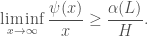
in the context of line $(3)$ . Our early estimates in Part II give $c \neq 0$ , whereby $\psi(x) \sim cx$ . It is an old result of Chebyshev that this forces $c=1$ (see the Exercises), and this concludes our proof. $\square$

— EXERCISES —

Exercise: Suppose that $\psi(x) \sim \alpha x$ for some constant $\alpha \neq 0$ . Show that this implies $p_n \sim \alpha^{-1} n \log n$ . Then, use Euler’s estimate on the harmonic sum of primes (given in the introduction) to prove that $\alpha =1$ . (While this was first noticed by Chebyshev in 1852, our work here shows that his result was well within the grasp of Euler, over a century beforehand.)

Exercise: Let $L=\{1,-2,-2\}$ , and use the closed form for $\chi_L$ to show that

$\displaystyle \sum_{k\leq \sqrt{n}}(-1)^{k-1}\psi(n/k)=n\log 2+O(\sqrt{n}).$

Use this estimate to give a second proof that $\psi(x) \sim \alpha x$ implies $\alpha =1$ . Hint: use the Taylor Series for $\log (1+t)$ .

Exercise: Use Bertrand’s Postulate to show that $L_n$ is never balanced, i.e.

$A(n):=\displaystyle\sum_{j \leq n} \frac{\mu(j)}{j} \neq 0$

for all $n >0$ . Similarly, show that the $n$ th harmonic number $H_n$ is never an integer. How does Möbius inversion connect these two results? Hint: For the first part, multiply by $n!$ and reduce modulo a large prime.

— REFERENCES —

[1] T. Apostol, Introduction to Analytic Number Theory, Springer (1976).

[2] P. L. Chebyshev, Mémoire sur les Nombres Premiers, J. Math. Pures Appl., 17, (1852).

[3] H. Diamond and P. Erdős, On Sharp Elementary Prime Number Estimates, L’Enseignement Mathématique, 26, (1980).

a. w. walker

mathematics and miscellany

Notes on the Chebyshev Theorem

Leave a Reply Cancel reply

Share this:

Like this:

Leave a Reply Cancel reply