Counting Real Quadratic Fields Without Unique Factorization

Let $k/\mathbb{Q}$ be a number field, i.e. a finite field extension to $\mathbb{Q}$ . We recall that the ring of integers in k, denoted $\mathcal{O}_k$ , is the ring

$\mathcal{O}_k := \{\alpha \in k : f(\alpha)=0 \text{ for some monic } f(t) \in \mathbb{Z}[t]\}.$

For $k= \mathbb{Q}$ , the ring of integers is just the integers $\mathbb{Z}$ , in which case we recall the Fundamental Theorem of Arithmetic: that every integer $n \neq 0$ may be written as a finite product

$n=\pm 1\cdot p_1 \cdots p_k,$

in which the $\{p_i\}$ are prime and uniquely determined (up to permutation). Domains for which this holds are known in general as unique factorization domains (UFDs). For $k = \mathbb{Q}(\sqrt{d})$ — with $d \neq 0,1$ square-free — the ring of integers $\mathcal{O}_k$ will in general not be a UFD. In fact, for $d <0$ , the integers $\mathcal{O}_k$ have unique factorization only in the 9 cases

$d=-1, -2, -3, -7, -11, -19, -43, -67, -163.$

Far less is known in the case $d >0$ (in which case k is known as a real quadratic field), although an unproven conjecture dating back to Gauss suggests that there should be infinitely many real quadratic fields. More recently, some heuristics stemming from Cohen suggests that the ring of integers in $\mathbb{Q}(\sqrt{d})$ should be a UFD with probability $\approx 0.75446$ as $d \to \infty$ on the square-free integers.

Here, we’ll focus on a more tractable variant of this problem:

Question: What can be said about the number $\tau(n)$ of distinct real quadratic fields $k=\mathbb{Q}(\sqrt{d})$ with $d\leq n$ for which $\mathcal{O}_k$ is not a UFD?

For a weak answer to the question above, we devote the rest of this article to the establishment of the following bound:

Theorem: As $n \to \infty$ , we have

$\tau(n) \gg \sqrt{n}\log n,$

in which the implied constant is made effective (e.g. greater than $1/11$ ).

For a high-level perspective, our plan is to identify a “large” infinite family of d for which the (images of the) norm forms in $\mathcal{O}_k$ are both uniformly well-behaved and restricted, in the sense that they can be chosen to uniformly avoid the norms of some select low-lying primes. To control the distribution of said primes (i.e. to ensure that they remain small), we trade power for control and restrict our study to the primes that ramify in $\mathcal{O}_k$ as opposed to those that split (which are far more numerous).

— PART I —

As always, we require a few Lemmas:

Lemma 1: Let $f(t) \in \mathbb{Z}[t]$ be of degree 2. Then the set

$P_f:=\{k: \vert f(k)\vert \text{ is prime}\}$

has natural density 0.

Proof: For any prime $p>2$ , we note that $p\mid f(n)$ for some n iff $f(t)$ admits a root in the finite field $\mathbb{F}_p[t]$ , which occurs precisely when

$\left(\frac{\Delta f}{p}\right)=0,1,\hspace{48 mm} (1)$

in which $\Delta f$ denotes the polynomial discriminant of f and $\left(\frac{\cdot}{\cdot}\right)$ denotes the Legendre symbol. Of course, this implies that $p \mid f(n+pk)$ for all integers k, and for $k\gg 0$ it follows that $f(n+pk)$ is composite. Thus, $p \mid f(k)$ on a set of density $1/p$ , and we have

$d(P_f) \leq \prod_{p \in A} \left(1-\frac{1}{p}\right),$

in which A denotes the set of primes such that (1) holds. Now, let $\Delta f= \pm 2^e \cdot m$ , in which $m >0$ is odd. (If $\Delta f =0$ , then $f(t)$ is reducible over $\mathbb{Z}[t]$ and our theorem holds trivially.) We have $(\pm 2^e \vert p)=1$ for all primes in a coset of $8\mathbb{Z}$ , and quadratic reciprocity implies $(m \vert p)=1$ for all primes in a coset of $m\mathbb{Z}$ . Thus A contains all primes in some arithmetic progression, and thus

$d(P_f)=\prod_{p \in A}\left(1-\frac{1}{p}\right)=\mathrm{exp}\sum_{p\in A}\log\left(1-\frac{1}{p}\right)<\mathrm{exp}\sum_{p \in A}\frac{-1}{p},$

which tends to 0 provided that the sum $\sum_{p \in A} 1/p$ diverges. This fact follows from the Chebotarev density theorem (or a sufficiently strong version of Dirchlet’s theorem on arithmetic progressions), and the well-known estimate $\sum_p 1/p =\infty$ . $\square$

Our second lemma concerns the density of square-free values for the polynomial $f(t) \in \mathbb{Z}[t]$ (as above). We define

$SF_f:=\{k:f(k) \text{ is square-free}\}.$

If $f(t)$ is assumed, we denote by $X(n)$ the set of roots of $f(t)$ over the ring $\mathbb{Z}/(n)[t]$ .

Lemma 2: Let $f(t) \in \mathbb{Z}[t]$ be of degree 2, with leading coefficient $a$ . Then

$\displaystyle d(SF_f)=\prod_{\substack{(\Delta f\vert p)=1\\ p\nmid a}} \left( 1-\frac{2}{p^2}\right) \prod_{p\mid (a\Delta f)} \left(1-\frac{\#X(p^2)}{p^2}\right). \hspace{14 mm} (2)$

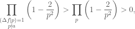
In particular, the density $d(SF_f)$ is positive iff the content $c(f)$ of $f$ is square-free and $f(t)\neq 2(t^2+t)$ .

Proof: Let $p>2$ be prime. As in Lemma 1, $p^2 \mid f(n)$ implies $(\Delta f\vert p)=0,1$ . If $(\Delta f \vert p)=1$ and $(a,p)=1$ , then Hensel’s Lifting Lemma implies that $f(t)$ admits exactly two roots over $\mathbb{Z}/(p^2)[t]$ . In particular, we have $p^2 \mid f(n)$ with probability $2/p^2$ as $n \to \infty$ . 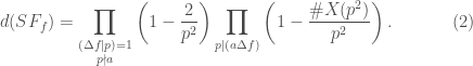If $p^2 \mid f(n)$ for some $p \mid (a\Delta f)$ , we find (likewise) that $p^2 \mid f(n)$ with probability $\# X(p^2)/p^2$ , and so the formula in (2) holds. As

$\displaystyle\prod_{\substack{(\Delta f\vert p)=1\\ p\nmid a}}\left( 1-\frac{2}{p^2}\right)>\prod_p \left(1-\frac{2}{p^2}\right)>0,$

wherein the last inequality follows from absolute convergence of the series $\sum_p 2/p^2 <2\zeta(2)$ , we have $d(SF_f)=0$ iff $\#X(p^2)=p^2$ for one of the finite primes dividing $a\Delta f$ . If $\# X(p^2)=p^2$ , then $f(t)$ admits $p$ roots over $\mathbb{F}_p[t]$ . For $p>2$ , this forces $f \equiv 0 \mod p$ (as $\mathbb{F}_p$ is a field and $\deg f <p$ ). Then $p \mid c(f)$ , and we repeat this argument for $f(t)/p \in \mathbb{Z}[t]$ to show $p^2 \mid c(f)$ . In the case $p=2$ , finite computation gives the stated exception, and these conditions are clearly sufficient for $d(SF_f)=0$ to hold. $\square$

Our final Lemma can be viewed as a strengthening of Lemma 1:

Lemma 3: Let $f(t) \in \mathbb{Z}[t]$ be of degree 2, and let $P_0$ be a finite set of primes. Let $G_f$ be given by

$G_f:=\{k \in SF_f : f(k) \text{ has a prime factor } p \notin P_0 \text{ with } p^3 < \vert f(k)\vert\}.$

Then $d(G_f)=d(SF_f)$ .

Proof: It suffices to show that the set

$S_f:=\{k :f(k) \text{ has a prime factor } p \notin P_0 \text{ with } p^3 < \vert f(k)\vert\}$

has density 1. Let $p$ be prime such that there exists an $n_p$ with $f(n_p)$ divisble by $p$ . Define $k_p$ such that 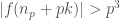$\vert f(n_p+pk) \vert >p^3$ for all $k>k_p$ (which exists as $\vert f \vert \to \infty$ ). As $p$ ranges across the primes in $A$ (where $A$ is as in Lemma 1), we have

$\bigcup_{p \in A} \left(n_p+pk_p\right)+p\mathbb{N} \subset S.$

As in Lemma 1, it follows that $d(S_f)=1$ . $\square$

— PART II —

In this section, we’ll begin to see how our Lemmas apply to the construction of real quadratic number fields without unique factorization.

Let $f(t) \in \mathbb{Z}[t]$ be of degree 2. Then $\sqrt{f(n)}$ is a quadratic irrational for any fixed $n \in \mathbb{N}$ , and so

$\sqrt{f(n)} =[a_0,\ldots, a_k, \overline{a_{k+1},\ldots, a_\ell}],$

in which the expression at right denotes the (periodic!) continued fraction expansion of $\sqrt{f(n)}$ . If the terms $a_i(n)$ can be taken as integer polynomials in $n$ , and if $k,\ell$ can be taken independent of $n$ (for $n$ sufficiently large), then we say that $f(t)$ has a uniform root. For example, $f(t)=t^2-2$ satisfies

$\sqrt{f(n)} =[n-1,\overline{1,n-2,1,2(n-1)}]$

for $n \geq 3$ and so $f$ admits a uniform root.

Theorem 1: Suppose that $f(t) \in \mathbb{Z}[t]$ of degree 2 admits a uniform root. As $n \to \infty$ , the ring of integers in $\mathbb{Q}(\sqrt{f(n)})$ fails to be a UFD for all n in a set of density $d(SF_f)$ .

Proof: Take $d>0$ square-free and set $k= \mathbb{Q}(\sqrt{d})$ . Let $\mathfrak{p} \subset \mathcal{O}_k$ be a ramified prime ideal, lying over the rational prime $p$ . If $\mathcal{O}_k$ is a UFD, then $\mathfrak{p}$ is principal (with generator of norm $\pm p$ ). For $d \equiv 2,3 \mod 4$ , the norm form in $\mathcal{O}_k = \mathbb{Z}[\sqrt{d}]$ is given by $x^2-dy^2$ , hence there exist integers $a,b$ such that

$a^2-db^2=\pm p. \hspace{47 mm} (3)$

If we suppose further that $p <\sqrt{d}$ , then (3) has a solution if and only if $x^2-dy^2=\pm p$ with $x/y$ one of the “pre-periodic” approximants to $\sqrt{d}$ (i.e. it suffices to check successive approximants up to $x/y=[a_0,\ldots, a_\ell]$ ; see here for more information).

If $f(t)$ admits a uniform root and $f(n) \equiv 2,3\mod 4$ , the approximants to $\sqrt{f(n)}$ appear as a rational function in $\mathbb{Z}(n)$ , and the norm form of the i-th approximation to $\sqrt{f(n)}$ takes the form

$\alpha_i(n):=a_i(n)^2-f(n)b_i(n)^2 \in \mathbb{Z}[n].$

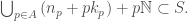
Let $P_0$ denote the (finite) set of primes $p$ which arise when $\alpha_i(n) =\pm p$ is constant. Otherwise, $\deg \alpha_i \geq 1$ , and we have $\sqrt[3]{f} \ll \alpha_i$ as $n \to \infty$ . For $n \in G_f$ sufficiently large, let $p < \sqrt[3]{f}$ be a prime divisor of $f(n)$ . Then the norm form fails to surject onto $\pm p$ , and $\mathcal{O}_k$ will not be a UFD by the remarks above. This proves our Theorem in the case $f(n) \equiv 2,3 \mod 4$ , and a proof for the case $f(n) \equiv 1 \mod 4$ is outlined in the Exercises. The result for general $f$ follows by consideration of the four polynomials $f(4t+i)$ , for $i=0,\ldots,3$ (each of which satisfies one of our conditions on $f$ ). $\square$

With this result in hand, we derive a (preliminary) lower bound on the function $\tau(n)$ . This is presented in the following example, which moreover sets the stage for our work in Part III.

Example: For $m>0$ , define $f_m(t):= m^2t^2+m$ . As

$\sqrt{f_m(n)} =[mn,\overline{2n, 2mn}]$

for all $n>0$ , it follows that $f_m$ admits a uniform root. Let $SF_m:=SF_{f_m}$ . As $c(f)=m$ , we note that $d(S_m)>0$ if and only $m$ is square-free. In either case, Theorem 1 implies that

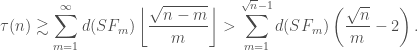
$\displaystyle\tau(n) \gtrsim \frac{d(SF_m)}{m} \sqrt{n}.$

To evaluate $d(SF_m)$ , we note that $\Delta f_m = -4m^3$ , so

$d(SF_m)=\displaystyle\prod_{\substack{(-m \vert p)=1 \\ p \text{ odd}}}\left(1-\frac{2}{p^2}\right)\prod_{p \mid 2m}\left(1-\frac{\# X(p^2)}{p^2}\right)$

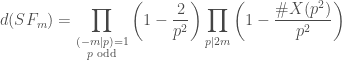
after some simplification. If we take $m$ square-free, then $\#X(p^2) \leq 2p$ for all $p \mid \Delta f_m$ (just consider the reduction into $\mathbb{F}_p[t]$ ). Now, if we define $\phi_2(n)= \prod_{p \mid n} \big(1-\frac{2}{p}\big)$ and $\rho:= \prod_p \big(1-\frac{2}{p^2}\big) \approx 0.322634$ , it follows that

$d(SF_m) >2\rho \cdot\phi_2(m)/m.$

For $m=1$ , we get the weak estimate $\tau(n)\gtrsim 2\rho \sqrt{n}$ . (With more care, this constant may be raised to $d(SF_1)=\prod_{p \equiv 1(4)} \big(1-\frac{2}{p^2}\big) \approx 0.894841$ .)

— PART III —

We now approach our final step in the proof that

$\tau(n) \gg \sqrt{n} \log n,$

which is achieved by (delicately!) adding the contributions of each $f_m$ to our lower bound on $\tau(n)$ . We require one more Lemma:

Lemma 4: If $f_{m_1}(n_1)=f_{m_2}(n_2)$ for any two $n_i >0$ , then $n_1 =n_2$ and $m_1=m_2$ .

Proof: We first note that $f_m(n) \in [(mn)^2,(mn+1)^2]$ for $n>0$ , since

$(mn+1)^2 =m^2n^2+2mn+1>m^2n^2+m =f_m(n)$

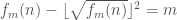for $n>0$ (and the lower bound is obvious). So $f_{m_1}(n_1)=f_{m_2}(n_2)$ implies that these values lie between the same perfect squares, i.e. $m_1n_1=m_2n_2$ . Yet $f_m(n)-\lfloor \sqrt{f_m(n)}\rfloor^2=m$ for all $n>0$ , which implies $m_1 =m_2$ (whence $n_1 =n_2$ ). $\square$

This “injectivity” result implies that we need not worry about double-counting our contributions to our estimate on $\tau(n)$ . We note that $f_m(t) \leq n$ provided that $t \leq \frac{\sqrt{n-m}}{m}$ , whereby

$\tau(n) \gtrsim \displaystyle\sum_{m=1}^\infty d(SF_m) \left\lfloor \frac{\sqrt{n-m}}{m}\right\rfloor > \sum_{m=1}^{\sqrt{n}-1} d(SF_m) \left(\frac{\sqrt{n}}{m}-2\right).$

(This step requires some uniformity in the rate at which $d(G_f)$ tends to $d(SF_f)$ , but this is not difficult, as $f_m \gg f_\ell$ for $m >\ell$ .) By introducing an error term (and slightly reducing our constants), this implies that

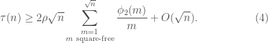
$\tau(n) \geq 2\rho\sqrt{n}\displaystyle\sum_{\substack{m=1\\m \text{ square-free}}}^{\sqrt{n}}\frac{\phi_2(m)}{m}+O(\sqrt{n}).\hspace{21 mm}(4)$

With this in hand, we are ready to prove our final estimate on $\tau(n)$ :

Theorem 2: As $n \to \infty$ , we have

$\tau(n) \gg \sqrt{n}\log n.$

Proof: To estimate the sum above in (4), we define the Dirichlet series

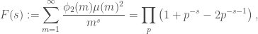
$F(s):=\displaystyle\sum_{m=1}^\infty \frac{\phi_2(m)\mu(m)^2}{m^s} =\prod_p \left(1+p^{-s}-2p^{-s-1}\right),$

where the introduction of the Möbius function is used to restrict our sum to the square-free integers. For $s>1$ real, we see that

$F(s) =\displaystyle \prod_p\left(1+p^{-s}\right)\prod_p \left(\frac{1+p^{-s}-2p^{-s-1}}{1+p^{-s}}\right)>C_3 \prod_p (1+p^{-s}),\hspace{4mm} (5)$

in which $C_3$ denotes the infinite product

$C_3:=\displaystyle\prod_p \left(1-\frac{2}{p^2+p}\right) \approx 0.471681.$

We recognize the rightmost product in (5) as an Euler product relating to the Möbius function, and so

$F(s) > \displaystyle C_3 \sum_{m=1}^\infty \frac{\vert\mu(m)\vert}{m^s}=\frac{C_3\zeta(s)}{\zeta(2s)}$

as $s \to 1$ along the positive axis. It follows that the N-th partial sum to $F(1)$ satisfies

$\displaystyle\sum_{m=1}^N \frac{\mu(m)^2\phi_2(m)}{m} \gtrsim \frac{C_3 \log N}{\zeta(2)}$

(by a consideration of the residue of $\zeta(s)$ at $s=1$ ), which yields to us the estimate

$\displaystyle\tau(n) \gtrsim 2\rho\sqrt{n}\cdot \frac{C_3\log \sqrt{n}}{\zeta(2)}=\frac{\rho \, C_3}{\zeta(2)} \sqrt{n} \log n$

using (4). $\square$

To get a handle on the constant appearing in the final estimate of this proof, we can unravel all of our infinite products. The resulting constant is then

$\displaystyle\prod_{p} \left(\frac{(p-1)^2(p+2)(p^2-2)}{p^5}\right)=\prod_p \left(1-\frac{5}{p^2}+\frac{2}{p^3}+\frac{6}{p^4}-\frac{4}{p^5}\right)$

$\approx 0.0925145 > \frac{1}{11}.$

Thus the implied constant in the statement of Theorem 2 may be taken in (slight) excess of $1/11$ , as earlier claimed. Without a doubt, this constant can be improved (perhaps with a more careful treatment of $\rho$ ).

— EXERCISES —

Exercise: As $f(t) \in \mathbb{Z}[t]$ varies over the polynomials of degree 2, show that $d(SF_f)$ can be made both arbitrarily large (less than 1) and arbitrarily small (while greater than 0). Is it the case that

$\{d(SF_f) : f(t) \in \mathbb{Z}[t] \text{ of degree } 2\}$

is dense in $[0,1]$ ?

Exercise: When $f(t) \in \mathbb{Z}[t]$ is of degree 2, what are the possible values of $\# X(p^2)$ ? Give necessary and sufficient conditions for each to occur. (Take care in the case $p=2$ .)